
The commercial feasibility must be assessed from two different points of view: lenders (the debt providers) and investors (the equity providers).
8.1.1 The Lenders’ Perspective (bankability)
The key aspect of the lenders’ concerns is the capacity of the project company to repay its debt on the agreed schedule.
To measure this ability, lenders usually define some criteria to judge a project’s bankability. Some of these criteria are the stability of project revenues, the ability of shareholders to provide collateral security (especially during the Construction Phase), and, particularly relevant to this section, the ratio between the cash resources generated by the project and the total amounts required to service debt. The most common ratios required by financial institutions are the following:
- Debt Service Coverage Ratio (DSCR): This ratio indicates the extent to which a project’s operating profits cover debt service obligations in each year[27] during the life of the contract. This ratio helps potential lenders determine the credit risk associated with the project. A higher Debt Service Coverage Ratio means that there is more operating surplus to cover debt service payments, and therefore less risk for lenders. Investors and lenders will expect a higher ratio in sectors that are perceived as risky. Maintaining a particular DSCR may also be a stipulation in a loan or bond covenant, and a decrease could trigger either an increase in debt service payments or some other legal remedy. The lenders will also stipulate a “lock-up” value (below which the DSCR should not fall) and a “default” value (below which the project company is considered to be in default). If the project’s DSCR falls below the lock-up value due to an insufficient cash flow, distributions to shareholders are prevented until adequate funds are available in order to allow the DSCR to return above the lock-up threshold. If default is reached, the lender can require its debt to be repaid or even take over control of the project (instead of the shareholders);
- Loan Life Coverage Ratio (LLCR). This ratio is commonly used in project finance. The ratio is defined as Net Present Value of Cash Flows Available for Debt Service (CFADS) divided by Outstanding Debt over the loan period. NPV (CFADS) is only measured up to the maturity of the debt. The ratio provides an estimate of the project’s credit quality from the lenders’ perspective; and
- Project Life Coverage Ratio (PLCR). The PLCR is the ratio of the Net Present Value of the Cash Flows Available for Debt Service (CFADS), available over the project’s remaining life, to the outstanding debt balance in the period. This ratio is similar to the LLCR, but in the LLCR the CFADS is calculated over the scheduled life of the loan, whereas the Cash Flows for the PLCR are calculated over the “project’s life”.
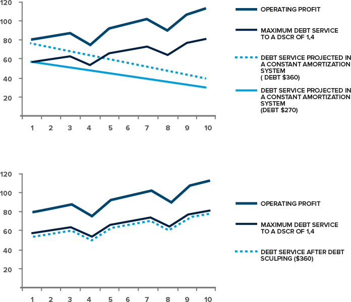
Despite of possible exercises that can be done in order to maximize the levels of debt in a project (see BOX 4.7), the ratios typically impose some type of cap for the amount of debt, given the capacity of the project to generate cash flow.
|
BOX 4.7: Debt Sculpting A common technique of financial modelling is known as Debt Sculpting. It consists of shaping the outline of debt repayment schedules in order to optimize the ability of the SPV to contract debt without violating the covenants imposed by banks, especially the DSCR. Consider, for example, a project with an estimated operating profit as shown below. The project would generate a steadily growing operating profit of around 5 percent a year, except in the years 4 and 8 in which reduced revenue is expected due to assets being partially closed for renewal. The project company is seeking finance with a bank that requires a minimum DSCR of 1.4. This covenant would impose a maximum limit of yearly debt service payments. The SPV is targeting a minimum of $360 in loans to be repaid in 10 years at a 10 percent interest rate a year. If the loan were repaid in the traditional constant amortization scheme[28], it would follow the outline below.
In this case, the debt being targeted of $360 would not be viable since it violates the covenant of DSCR = 1.4 in years 1 through 4. In fact, only a debt of $270 or lower could effectively be contracted while respecting the covenant imposed by the bank and the Constant Amortization System. However, the financial advisors can carry out Financial Sculpting by trying to increase the level of debt of the same project. Considering the same assumptions of interest rates of 10 percent a year and the same repayment term, this would lead to the following debt outline for the desired $360 of debt. (Refer to the 2nd graph above). Debt Sculpting can allow a higher amount of debt to be raised in the same project, thus maximizing the commercial viability of the project (see section 8). |
The effective thresholds depend on the market conditions of each country and sector. Thus, these should be approximated in order to assess the commercial feasibility of the base case from the lenders’ perspective, which may be done with the support of the financial advisor and/or be based in recent and similar project precedents.
The fact that the project can incorporate the required level of debt, however, is not enough to classify it as commercially feasible. The capacity of the project to remunerate the equity investors is also paramount if the project is to attract bidders.
8.1.2 The Investors’ Perspective
For an equity investor, a project must be both bankable and provide an acceptable return for the risk of the investment. The two most common techniques used to assess the commercial feasibility, from the investors’ perspective, are the calculation of the Net Present Value, based on the discounted equity cash flow, and the internal rate of return of the equity cash flow. Both techniques are based on the assumption that, for a project to be considered commercially viable, the investment must provide a return over time for at least as much as an alternative and comparable investment[29].
The Net Present Value of the equity is the sum of the investor’s future cash flow in today’s values, and it can be demonstrated by the following formula:
![]()
Where:
- NPV = the Net Present Value or the sum of the equity cash flow values in today’s currency;
- CFt = the net equity cash flow value resulting from each period’s revenues, expenses, debt service, and other parameters defined in the model;
- i = the discount rate or the cost of capital for equity investors over time;
- t = the number of the period in which the value is being discounted, and
- n = the total number of periods in the cash flow.
The NPV is a representation of the present value generated by the project above the returns represented by the discount rate. So, if the NPV is above zero, it means the project will generate value to investors above the required rate of return. For example, if an NPV discounted with an annual discount rate of 8 percent is above zero, the average yearly rate of return of the project is higher than 8 percent. Conversely, if the NPV is negative, the project offers a return on the investment lower than 8 percent. If the NPV equals zero, then the yearly average return on equity investment will be exactly the percentage used as the discount rate.
The most common use of NPV as an assessment of the Equity Cash Flow is to test if its value is positive, in which case the project is deemed viable from the investor’s perspective, as long as the discount rate used is the return on the capital required by the investor, as the minimum threshold.
Another methodology, which is very similar in principle with the NPV calculations, is the Internal Rate of Return (IRR)[30]. Mathematically speaking, the IRR is the discount rate that makes the NPV of any given cash flow equal zero. In other words, the IRR is an output of the cash flow that indicates the return offered by the project on the invested amount, and it is the preferred technique by many financial advisors.
So, if the equity IRR of the equity cash flow is higher than the required rate of return of the investors (sometimes called a hurdle rate), a project is said to be commercially attractive. If the IRR is lower than the required return, the project is not viable.
Both techniques demand the estimation of the rate of return required by investors as the minimum threshold below which the project is not commercially feasible.[31]
The estimation of an equity investor’s required rate of return, or the cost of equity, is not a trivial task. In theory, some of the factors that affect the required rate of return for a specific project are as follows.
- The higher the project’s specific risks that may affect the expected cash flow are, the higher the return on equity required by investors;
- The higher the systemic risks associated with specific sectors that can affect the cash flow or the regulatory stability of the contract are, the higher the return on equity required by investors;
- The higher the country risk perceived by the investor, the higher the return on equity required by investors;
- The higher the return obtained for investments with similar risk profiles, the higher the return on equity required by investors; and
- The more guarantees offered by the government that reduce the volatility of the cash flows, or limit the impact of political risk, the lower the return on equity required by investors.
To incorporate these trends in the model in order to estimate an appropriate rate of return requires specialized knowledge. A common way of setting the cost of equity, or the return on capital required, is to review the return levels requested by investors in previous projects similar to the one that is being analyzed (or at least other infrastructure projects in the country with similar risk levels). This information is usually unavailable to the public, so information from advisers can play an important role. In cases in which information on similar projects is not available, a small market test with potential project investors can be useful. Finally, if none of the previous alternatives are possible, the minimum return can be estimated through the use of the Capital Asset Pricing Model (see box 4.8).
|
BOX 4.8: Capital Asset Pricing Model (CAPM) The Capital Asset Pricing Model studies the cost of equity of publically traded companies (also known as “listed” companies). By analogy, the results obtained can be applied to other companies, even if they are not listed, since they have similar risks to those of listed firms. According to this methodology, the cost of equity (Ke) can be estimated as the return on a riskless asset plus the “market risk premium” adjusted to reflect the volatility of the investment compared to the volatility of the market. The general expression of this model is provided by the following equation:
Where: Ke = Cost of Equity Rf = Return on a riskless asset b = Volatility of the analyzed company in relation to the market Rm = Market return To estimate the return on a riskless asset, it is common to use the interest rate on public debt (using a debt issuance/bond with a term as close as possible to the contract period being analyzed). Market returns can be obtained from the stock market’s data on the returns of companies managing infrastructure similar to the project being analyzed. The volatility coefficient (b) measures the variation of the company’s performance with respect to changes in market performance. The beta is usually estimated by regressing the historical stock prices of companies that manage similar infrastructure in the market. Source: The Municipality of Rio PPP guide: Screening, Appraisal and Auctioning of PPPs (Volume 2, Section III) |
An IRR equal to or higher than the required equity rate of return, or an NPV equal to or greater than zero, represent the most commonly used financial indicators to evaluate the quality of a cash flow from the investor’s perspective. There are other aspects, however, that can be relevant decision drivers for investors analyzing a project’s cash flow.
- The project IRR, considering the return of the Project Cash Flow as opposed to the Equity Cash Flow. This can be an important indicator of the quality of the cash flow of the project as a whole, and thus is a determinant of the enterprise value (this can be used to estimate the market value of the stock of the Project Company in case an exit strategy is considered by investors);
- The nominal or discounted payback period which represents the period required before the accumulated cash flow equals zero, respectively, in nominal or discounted terms. Generally, the longer the payback period, the higher the risks perceived by investors; and
- The absolute size of the investment. This variable can be a key decision driver because it might rule out several equity providers, even in the case where a very attractive IRR is provided by the project. Some investors might not be able to provide the required amount of equity subscription because it is too large, while others might have a policy not to invest if the equity required is below a minimum threshold.
Taken together, the estimation of these financial indicators, as well as the analysis of bankability, allow the project team to observe the project from the private sector’s perspective, which is an essential exercise in order to guarantee that a commercially feasible project will eventually be launched to the market.
[27] The period of analysis can be shorter than one year.
[28] In the example, a Traditional Constant Amortization Scheme is used to refer to a debt repayment outline in which the principal is repaid in linear amounts in each period. The interest incurred is then paid fully in each period. Since the debt balance is decreasing, the interest also decreases steadily through time. So the total debt repayment value also decreases.
[29] E. R. Yescombe’s book PPP: Principles of Policy and Finance (2007) presents the private sector’s perspective on PPP financial issues, including detailed analysis about several value drivers for investors. See chapters 7, 8 and 9.
[30] One of the problems with the use of the IRR is that its mathematical structure assumes the cash outflows are reinvested at the same rate as the calculated IRR. Since this might not be a reasonable assumption, an alternative method commonly used is the Modified IRR (MIRR). The MIRR function allows inputting the rate of reinvestment separately and thus calculating the effective return offered by the project. For a discussion on the limits of the IRR and the use of MIRR, see Yescombe’s book Public-Private Partnerships: Principles of Policy and Finance (§4.4.2).
[31] The Rate of Return required by investors is different, generally higher, than the cost of capital of the government or the rate used by government to compare different investment initiatives.
Add a comment